
Refractory materials are required to keep their structural stability when subjected to extreme mechanical and chemical environments. Thermal shock spalling, corrosion, creep, and other complex phenomena may take place while using them. Therefore, mechanical behavior of refractory materials is of great interest.
In recent years, researchers reported various technical problems and industrial challenges concerning refractory materials that are not easily solved using conventional experimental methods. Thus, numerical computational tools emerged to better understand the physical problems and to analyze such complex conditions.
The finite element method (FEM) is one of the most popular approaches for studying thermomechanical problems. It is a numerical method that subdivides a large system into smaller, simpler parts for easier analysis through the use of a mesh, i.e., a geometrical representation of the domain of interest that comprises all elements to be analyzed.
This technique is suitable to solve elliptic and parabolic problems, and it is not restricted to linear or isotropic cases. The mesh makes it geometrically flexible and able to model complex domains. Additionally, this technique is easily implemented as computer codes and is also robust because most mathematical problems can be stated as a variational problem where FEM can be applied. However, one of the main disadvantages to FEM is the difficulty of analyzing microscopic situations and material discontinuities, as the equations associated with the problem are derived based on a continuous materials assumption.1
Trying to overcome this issue, researchers developed the FEM remeshing technique, which solves complex problems by updating the mesh to consider discontinuities, but this procedure can affect its performance.2 Möes et al.3 developed the extended finite element method (XFEM) to model fracture and interfacial problems, using discontinuous basis functions on the nodes where cracks may occur. The advantage of this procedure is that it is not necessary to update the mesh. Nevertheless, this method also has a high computational cost and the study of complex features, e.g., crack initiation at multiple locations, is still an ongoing research.1
In contrast to FEM, meshfree methods have been studied, developed, and proposed as an alternative approach. Some examples are the smoothed-particle hydrodynamics (SPH) and its modified approach (corrective SPH and discontinuous SPH),4 the moving least square (MLS),5 and the element-free Galerkin method (EFGM).6 These techniques aim to study a problem with a random distribution of nodes without a mesh or connection between them. Nevertheless, they are very time-consuming and may undergo several numerical issues, such as low accuracy near the boundaries and difficulties to impose Dirichlet boundary conditions.1
Another approach to modeling discontinuous problems is through discrete methods, such as molecular dynamics (MD)7 and the discrete element method (DEM).8 These methods differ from FEM because the body is not represented by a continuous mesh where constitutive laws are obeyed but rather by a set of discrete bodies or particles that interact with its neighbors following contact or distant interaction laws at the microscale.
Such interactions create emergent properties that can be measured on a macroscale as an apparent property that results from the multiple interactions at the microscale. This possibility enables DEM to be a tool with great potential for modelling cracks and representing microstructures that have a large number of discontinuities, such as inclusions, cracks, debonding, and porosity, which is the case of refractory materials. In addition, the major advantage of DEM is the likelihood of investigating both crack initiation and propagation, as well as the phenomena of coalescence and bifurcation, which can be used to understand and simulate the macroscopic behavior of the materials9 (Figure 1).
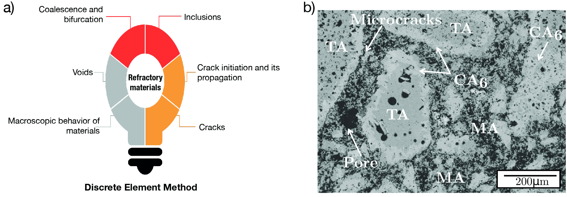
Figure 1. (a) Schematic representation of features of a refractory material and its connection with DEM, (b) SEM micrograph of a spinel containing alumina castable refractory showing all multiple phases, pores, and microcracks. (TA: tabular alumina; CA6: CaO.12Al2O3; MA: MgAl2O4) Credit: Moreira et al.
Various studies used DEM for ceramics applications (continuous problems), regarding problems related to compression tests,10 crack initiation and propagation in alumina,11 and the effect of average grain size on the toughness of alumina ceramics.12 André et al.13 studied the Young’s Modulus of a borosilicate glass matrix with alumina inclusion affected by microcracks. Wang14 analyzed the fracture propagation in concrete to evaluate the difference in strength due to aggregates and aggregate/mortar interfacial transition zone (ITZ), yielding insights concerning the effect of the microstructure on its mechanical behavior.
Nevertheless, DEM has not been extensively applied to model commercial refractory materials, although it can improve the link between the material’s microstructure (which has a large number of discontinuities) with their macroscopic properties during application.13 Such approach can optimize the processing and applications of refractory materials, increase their performance, and save time, effort, and resources in the industry.
There are two major challenges to applying DEM for continuous problems: the choice of the contact model between the particles and how to find the corresponding microscopic parameters that describe the macroscopic behavior of the material (the calibration step). The present work is based on previous research that proposed a straightforward approach to overcome such challenges.9
The aim of this study was to explore the possibilities of applying discrete element modeling as a tool for analyzing mechanical tests of refractories. The results attained can lead to models that in the future could help global key players to overcome, for example, the challenges of evaluating the mechanical and thermal damage in steel plant installations, which are not easily developed experimentally.
Thus, an alumina castable considering Alfred’s grain size distribution was studied with GranOO, an opensource discrete element workbench.15 The calibration process was carried out by an automatic algorithm developed by Andreá et al.9 and by a manual calibration accomplished using the Brazilian and uniaxial compression tests. The three-point bending test was used in a further validation step.
Materials and methods
Discrete element method (DEM)
DEM is fundamentally different from continuum methods, such as FEM. Instead of considering the regions of interest as a continuum media, where known constitutive laws describe its behavior in a grid (the domain’s mesh in FEM), in DEM the domain of interest is expressed by a set of rigid spherical bodies that interact following specific laws.1
For the representation of mechanical phenomena, DEM, which originated as a tool for simulating naturally discrete problems such as granular flow, powder compaction, and related problems, can be of great benefit when specifying laws of bonding between elements.16
The bond between particles can be based on distinct models. The most common ones are the contact bond (simple spring) model, the dual spring model, the parallel bond and flat joint models,16 and the recently developed cohesive beam model.9 Figure 2 presents a schematic representation of some common bond models.
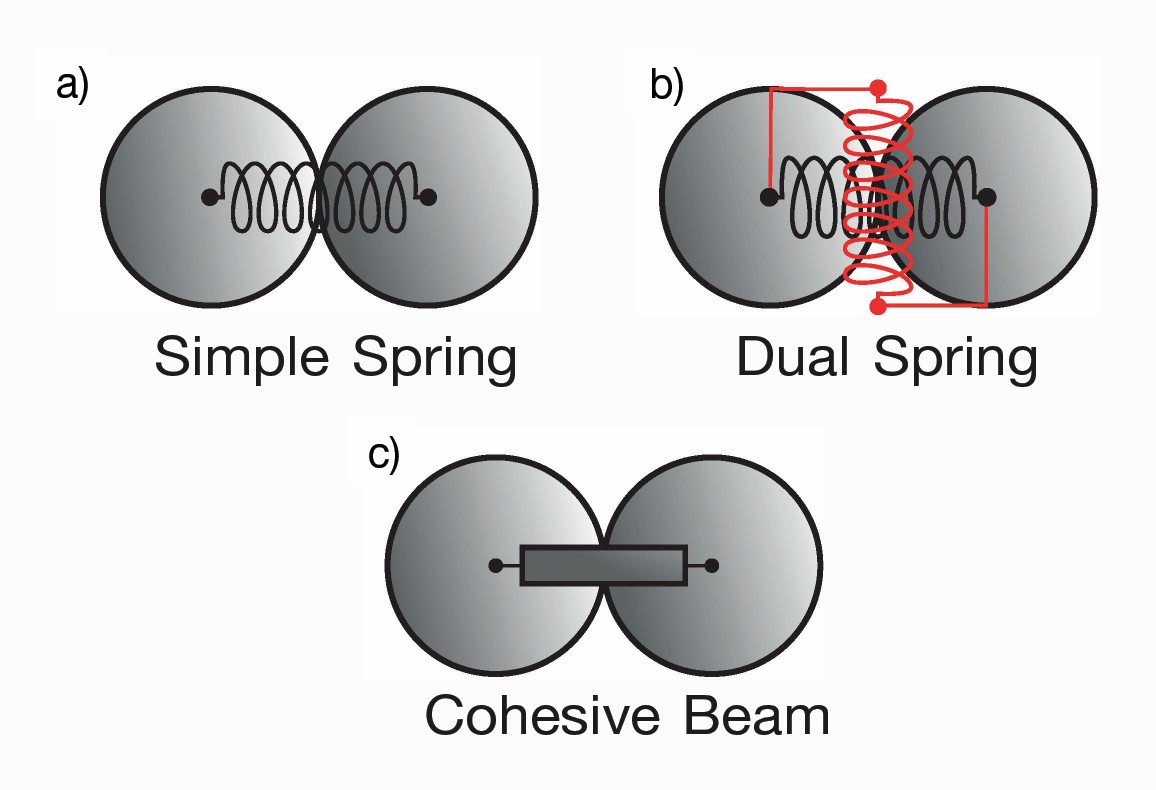
Figure 2. Schematic representation of the most common cohesive bond models. Recreated from Reference 1. Credit: Moreira et al.
Each bond model is characterized by a set of variables, which are commonly referenced as micro (or local) parameters. Because the mechanical behavior of the whole structure is an emergent property that arises from the interaction of each element, two distinct scales are separately considered: the macroscopic (the scale of the material sample that will be simulated and is represented in the model) and the microscopic (the discrete element scale), as seen in Figure 3a.
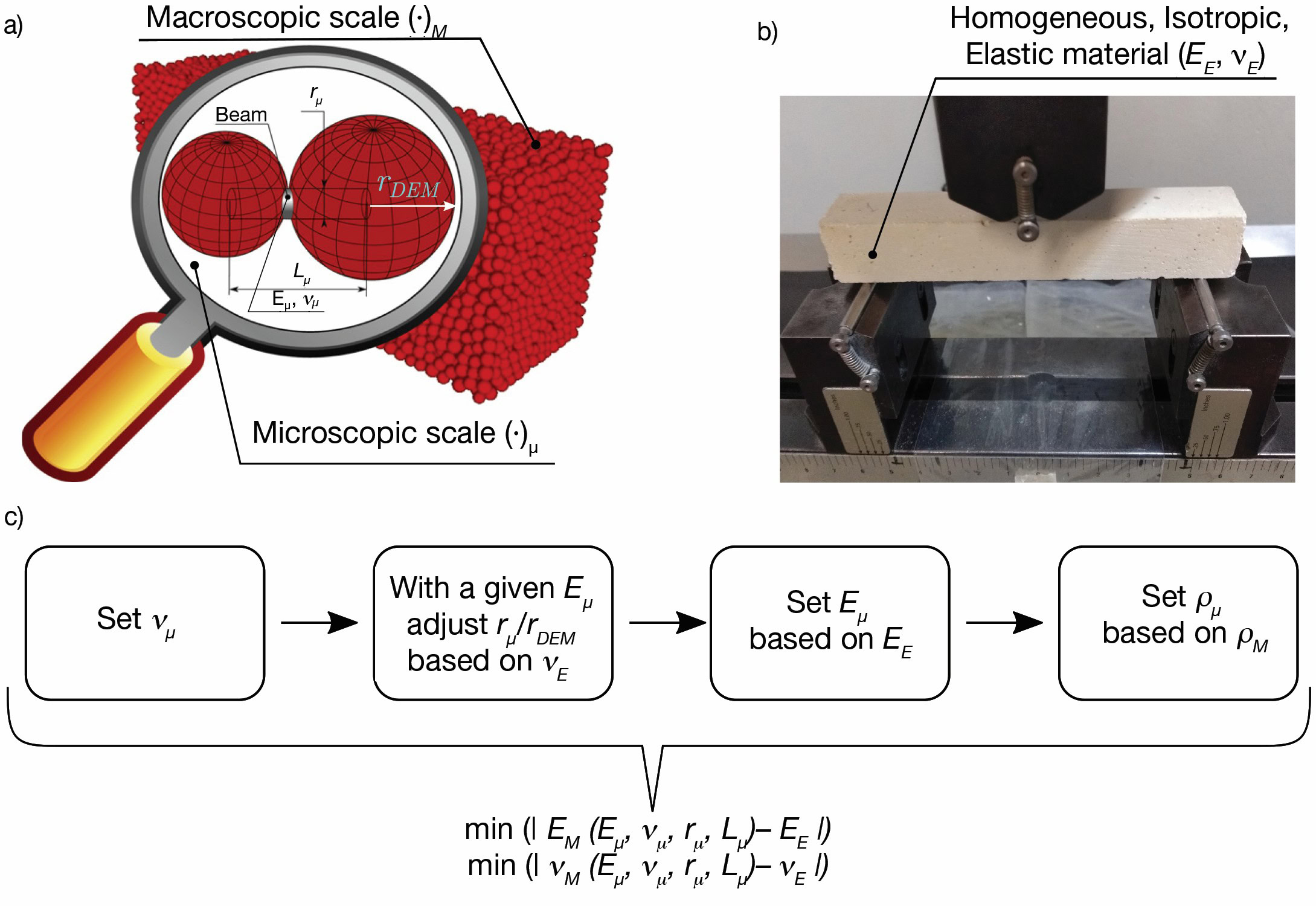
Figure 3. Common procedure for a DEM simulation. a) Describes both scales and the cohesive beam model and its properties, including the beam’s length (Lμ), its radius (rμ), the Young’s Modulus (Eμ), and the Poisson ratio (νμ). b) Shows the actual sample and the assumptions made (an elastic material described by its Young’s Modulus (EE) and the Poisson ratio (νE). c) Presents the automatic calibration algorithm used and its mathematical meaning, the minimization of the difference between simulated macro properties and the experimental ones (adapted from Reference 1). Credit: Moreira et al.
The physical features of the whole sample are referenced as macroscopic properties, whereas the quantities related to the bonds and individual elements are the already mentioned microparameters. Although studies were conducted in order to propose analytical relationships between the set of micro- and macroparameters,17,18 there are no direct laws that correlate the set of microparameters and the experimentally measured properties of the material.17
Thus, a calibration step is commonly needed to find the set of microvalues that best represent the mechanical behavior (Figure 3c). Usually, experimental tests with a homogeneous stress state, such as uniaxial compression, are used for the calibration step, whereas an experimental one with a nonhomogeneous stress state is applied to validate the model obtained with the optimal set of microparameters.18
GranOO workbench
The Granular Object-Oriented workbench (GranOO) was used for the DEM simulations. GranOO is not a software but rather a set of C++ libraries that was originally developed to study tribological problems,19 and it was redesigned in order to be generalized and used in multiple DEM simulations. Based on the open source nature of this project, any contact bond model can be implemented; however, a default cohesive beam model is available, which is described by the beam’s properties: Lμ , rμ , Eμ , and νμ (Figure3a). The fundamental idea is to use the Euler-Bernoulli theory of beams to express their mechanical behavior.
GranOO workbench also has an algorithm solution for the creation of the DEM domain. This step is important as there are three properties for the geometric representation of the domain that should be assessed in order to have DEM models for continuous materials: the homogeneity, the isotropy, and the fineness. Further details can be found in André et al.19
Next, GranOO also presents an algorithm for the automatic calibration of the microparameters. This algorithm is based on a number of quasistatic tests carried out in a model material and is fully described by André et al.9 This algorithm minimizes the difference between the macro properties that arises from the DEM model and the experimental properties, as described in Figure 3c.
The last step is a dynamic calibration of the density of the discrete elements to ensure that the overall mass of the DEM domain equals the continuous body density, compensating the virtual porosity due to the spherical shape of the DEM elements.9 Finally, a failure criterion needs to be set for the DEM model to define the bond breakage, thus the approach used on the GranOO workbench and the manual calibration procedure.
Failure criteria and manual calibration
The discrete nature of DEM makes it a good candidate for modeling the failure of materials. However, a failure model needs to be defined in order to have a qualitative comparison with the experimental results.1 There are two major classes of approaches to model a fracture within the DEM framework: a local description (in the cohesive beam) and a nonlocal one.
Both methodologies were compared, and the nonlocal description was found to better represent the behavior of the failure of brittle materials, both at a micro- and macroscale. This approach consists of using the virial stress and converts it into the equivalent Cauchy stress tensor for each discrete element, taking into account its interaction with each neighbor.1 Finally, any of the common failure criteria, e.g., hydrostatic, von Mises, Tresca, Rankine, or Griffith, can be considered using the Cauchy stress tensor of each discrete element.
The present work uses the Rankine criterion for the results obtained via GranOO’s automatic calibration algorithm. In addition, another approach was applied in the current work using an asymmetric Rankine criterion in both tension and compression defined as σ1 > σμ,t or σ3 < –σμ,c (considering the three principal stress σ1 > σ2 > σ3). However, as already described, both limits of microstress in tension (σμ,t) and compression (σμ,c) need to be calibrated, leading to a second group of results. Such limits were obtained by applying a fixed set of microparameter values and a manual calibration of σμ,t and σμ,c using the Brazilian and the uniaxial compression results, validated by a three-point bending test. All three experiments are commonly used for mechanical characterization of refractories.
Experimental procedure and modeling assumptions
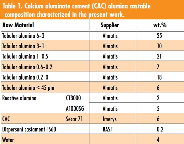
A 6 wt.% of calcium aluminate cement alumina castable (Table 1) was developed to assess DEM, following Alfred’s Packing Model (q = 0.26). The samples were molded as cylinders (40 mm in diameter and 40 mm in height) for the Brazilian test, cylinders (50 mm 3 50 mm) for the uniaxial compression test, and as bars (25 Χ 25 Χ 150 mm³) for the three-point bending test.
The experiments were conducted following ASTM C133 for the three-point bending test and the uniaxial compression measurements, using universal testing systems MTS (MTS810, MTS Systems Corp) or Instron 5500R, respectively. The Brazilian test was carried out with a fixed displacement of 1.3 mm/min and parallel plates as supports. All samples were evaluated after curing for 24 hours in a climate chamber with 80% of relative humidity and dried at 110°C for another 24 hours.
To reproduce the mechanical tests, constant displacements were fixed on positions of the DEM domain in a manner to simulate the experimental conditions (Figure 4). The explicit dynamic algorithm of GranOO automatically computes an optimal time step and the displacements are defined per increment. For the current work, the displacement used was 2 Χ 10–9 m/iteration.
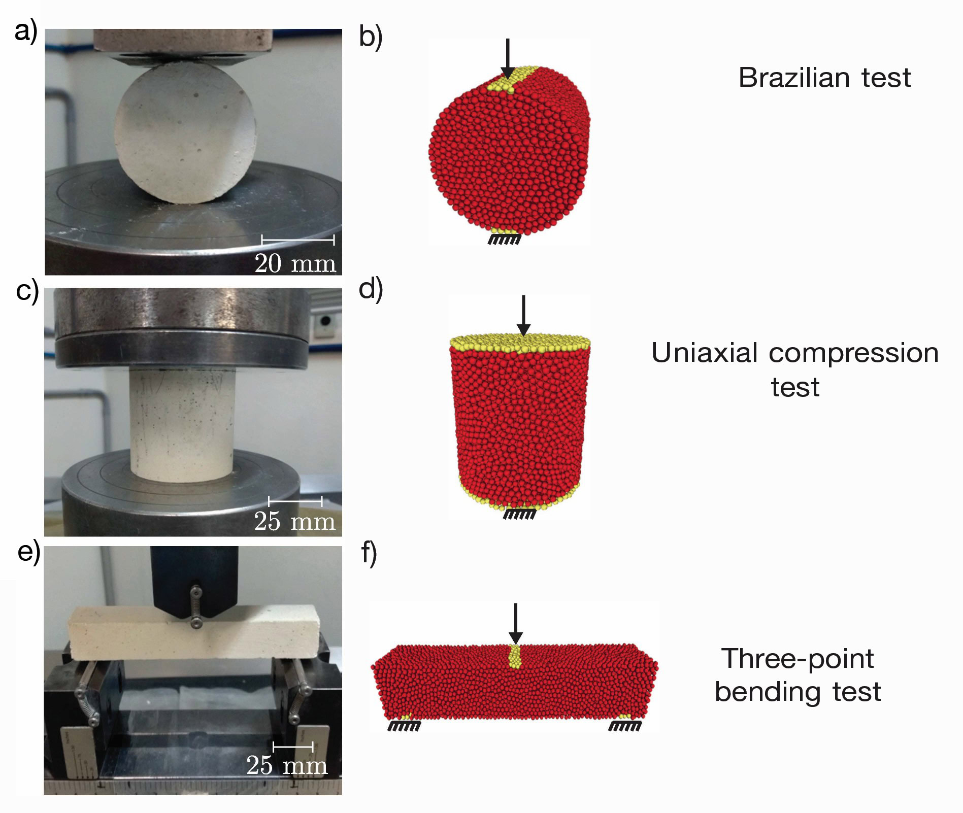
Figure 4. Experimental setup (a), (c), and (e), and DEM representation, (b), (d), and (f). The yellow discrete elements represent the set that will be displaced (black arrows) or clamped (black fixed support). Credit: Moreira et al.
The material is considered homogeneous, isotropic, perfectly elastic, and brittle on the simulations. Such assumptions are considered reasonable when considering the experimental results of the mechanical tests.
Automatic calibration results
Each experimental test was reproduced in discrete element domains of the same dimensions of the real samples. The macroparameters used were: Young’s modulus of 62.04 GPa measured with an optical extensometer (Instron AVE 2663-821) on a uniaxial compression test equipment (Instron 5500R), Poisson ratio of 0.25 measured by impulse excitation technique (Sonelastic), and tensile failure strength of 9.06 MPa (measured by the Brazilian test).
Brazilian test
This test yields a tensile stress state in the samples that generates cracks from the middle of the cross section to the loading contact of the machine.20 There are also shear failures in the regions close to the loading area. Figure 5 shows the crack propagation evolution and a picture of the experimental sample failure after the Brazilian test.
The crack propagation in the numerical model (Figure 5a-d) agrees qualitatively with the proposed description of the tensile and shear failure mechanisms. In Figure 5e, the photograph shows the failure of an experimental sample that presented the expected crack pattern.
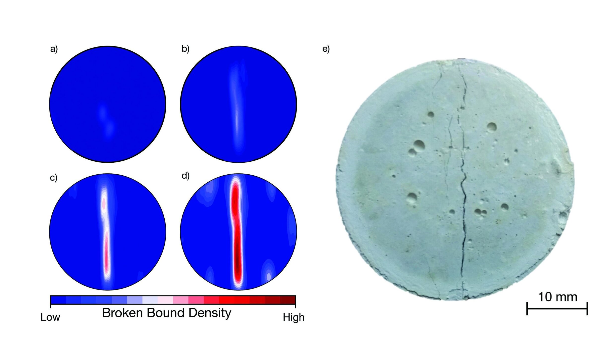
Figure 5. (a-d) Results for the Brazilian test broken bounds density progress and (e) photograph of the tested sample failure. Credit: Moreira et al.
Three-point bending test
The three-point bending test results can be analyzed in Figure 6. In (a-d), the crack originates between the lower loading rods, in the region where the tensile stress is the highest. This qualitative benchmark is important as it agrees with the results observed experimentally.
In Figure 6e, the comparison of the numerical and experimental force-displacement curves shows a good agreement between the macro Young’s modulus for the linear regime of the experimental curves. The experimental results considered a correction factor due to the loading device deformation, however, the precision of such experiment could be improved with the aid of digital image correlation (DIC), which could provide a more accurate description of the actual behavior of the material. Nevertheless, there is a difference of 16.2% regarding the loading failure, which could be related to the Rankine failure criterion used for the automatic calibrated simulations.
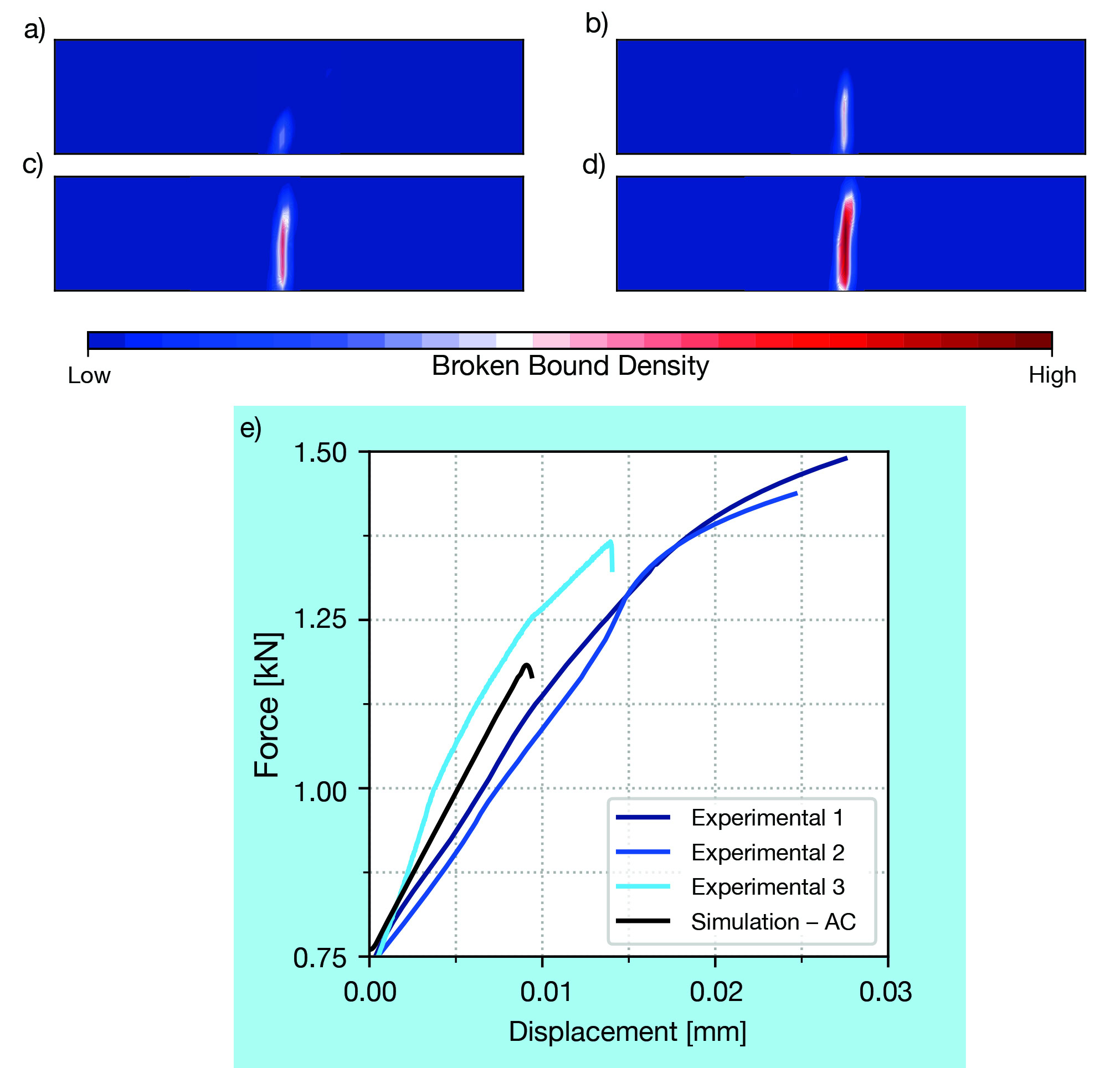
Figure 6. (a-d) Results for the three-point bending test broken bound density progress and (e) force-displacement curve for the simulation and the experiments. Credit: Moreira et al.
Uniaxial compression test
For this test, a homogeneous compression stress state that can yield two main types of failures was assumed: shear failure or columnar vertical failure. The model crack propagation pattern did not yield insightful analyses, thus Figure 7 only presents the stress-strain curve that was assessed with the aid of an optical extensometer.
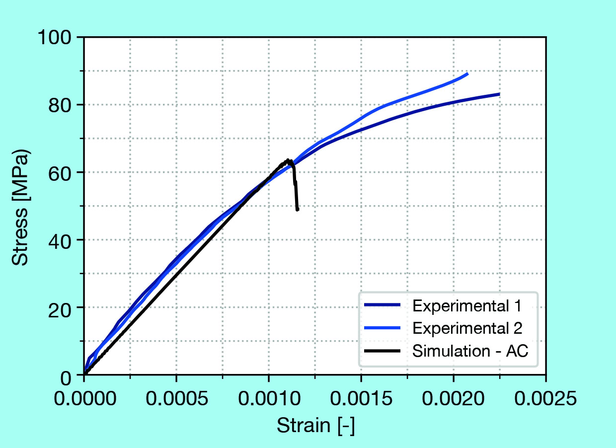
Figure 7. Stress-strain curve for the simulation using the automatic calibration (AC) and the experiments. Credit: Moreira et al.
The comparison between numerical and experimental results show a good agreement for the Young’s modulus, but the macrostress at failure is 29.0% lower for the DEM simulation. This finding could be related to the model assumptions, the shear effects not captured on the model, or the Rankine criterion used to define the breakage of the cohesive beams.
Manual calibration results
The user defined criterion is defined by two distinct conditions, one for the maximum principal tensile stress, σ1 > σμ,t, and another for the maximum compressive stress, σ3 < –σμ,c. The limit values were calibrated using the Brazilian test, which yield a good agreement, and the uniaxial compression one, which showed the largest difference in the experimental results. The calibrated criterion is validated with the three-point bending test. All the other microparameters were set equal to the values of the automatic calibration for the Brazilian test.
Calibration process of failure criterion
In order to calibrate this user defined criterion, multiple simulations with values of σμ,t ∈ [7 MPa, 14 MPa] and σμ,c ∈ [40 MPa, 210MPa] were carried out. The calibrated values were σμ,t = 13.5 MPa and σμ,c = –200 MPa. Using them for the user defined criterion resulted in a macro failure load which was within an error of 9.7% for the Brazilian test and 6.3% for the uniaxial compression one.
Three-point bending validation
The three-point bending DEM simulation using the calibrated values for the limits of the failure criteria can be found in Figure 8b. The values for the automatic calibration are also presented, highlighting that the new failure criterion still describes the mechanical behavior in a similar way to DEM simulation obtained from the automatic calibration, with the advantage of reproducing the uniaxial compression results. The difference between the experimental value of failure load is 2.27%, which is lower than the result for the automatic calibration, 16.2%.
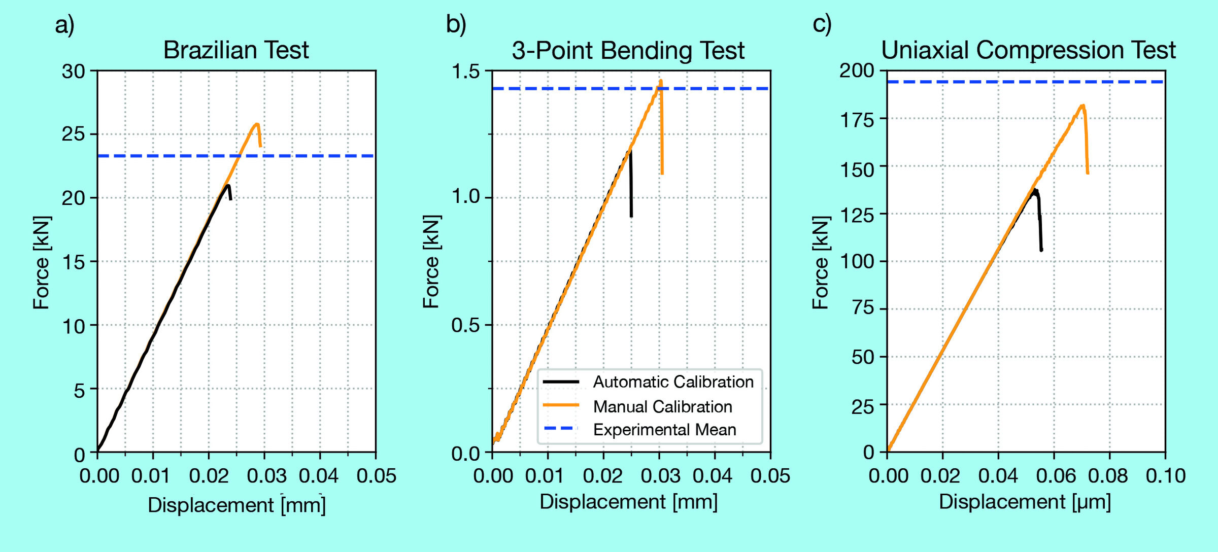
Figure 8. Results for the automatic and manual calibration and the average of the experimental results for the (a) Brazilian, (b) three-point bending, and (c) compression tests. Credit: Moreira et al.
Conclusions
In the present work, a first “plug and play” approach using GranOO and its automatic calibration algorithm for the microparameters yielded promising results, when considering the crack patterns and the Young’s modulus. However, the failure load errors were between 15–30%.
To address such inconsistency, a user defined failure criterion was investigated, and a manual calibration using the Brazilian and uniaxial compression test resulted in a model capable of reproducing the mechanical behavior of the three-point bending test both qualitatively (crack path) and quantitively (Young’s modulus and load at failure).
The simulations were carried out on a regular desktop with a third generation Intel i5 – 3570, which shows the feasibility of such models for more complex geometries. It should be noted that more advanced experimental setups, such as using strain gages for the other tests besides uniaxial compression and digital image correlation, could be of great interest in order to have more reliable data for the comparison with the numerical results.
Using DEM highlighted important challenges that should be overcome to make it a reality. Namely, the crack propagation behavior for the compression test, the displacement values, and an approach to have a good match between the micro and macro properties only based on quantities with physical meanings.
Above all, the present work showed the potential of this tool to aid in materials design by modelling real microstructures of refractories (considering pores, particle size distribution, morphology of the grains, different phases, and more). This modeling can lead to the assessment of the local strength of the material, especially when considering complex geometries and phenomena, such as the drying of monolithic refractories, thermal shock, creep, and even bioinspired microstructures.
Acknowledgments
The authors would like to thank Dr. R. Angélico (Aeronautical Engineering Department at the University of São Paulo in Brazil) for the technical discussions and F.I.R.E., Tata Steel Netherlands, CAPES, and CNPQ for providing resources to carry out this work.
Capsule summary
Modeling discontinuities
Discrete element modeling, which models interactions of discrete particles, can model microstructures with a large number of discontinuities, such as refractory materials.
Challenges to DEM
DEM faces two challenges modeling continuous problems: choosing a contact model between particles and finding corresponding microscopic parameters that describe a material’s macroscopic behavior.
A manual fix
A manual calibration using Brazilian and uniaxial compression tests results in a DEM model capable of reproducing the mechanical behavior of a continuous problem.


Related Articles

Bulletin Features
The nonferrous metals market: Supply and regulatory pressures inspire strategies for a resilient future
Nonferrous metals serve foundational roles in the electrification, renewable energy, and digital transformation. Nonferrous metals are metals that do not contain iron in significant amounts. These metals typically are nonmagnetic, corrosion resistant, electrically and thermally conductive, and lightweight, making them ideal for applications in the emerging markets mentioned above. Even…

Market Insights
Industrial digitalization: ‘Smart’ operations can improve worker safety and well-being in high-temperature environments
Heavy industry is the backbone of economies around the world, critical to automotive production, construction, the energy sector, and everything in between. But many heavy industries are facing worker shortages. There are more than 400,000 open manufacturing jobs in the United States, according to the Bureau of Labor Statistics.1 With…

Market Insights
‘Fail fast’ manufacturing: How disciplined experimentation strengthens, not threatens, quality
In manufacturing, few phrases raise eyebrows faster than “fail fast.” In the startup world, this business strategy is celebrated as a sign of agility. On a ceramic manufacturing floor, it can sound careless or even dangerous. In manufacturing, few phrases raise eyebrows faster than “fail fast.” In the startup world,…